Highly Nonlinear Approximations for Sparse Signal Representation

• Project Overview
• Tutorial [.ps | .pdf]
• Source code
• Examples
• Publications
• EIFS
• SCEIFS
• Acknowledgements

• Home
• maths@Aston
• EPSRC Home

Managing the constraints

Without loss of generality we assume here that the measurements on the signal in hand are given by the values the signal takes at the sampling points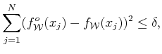 $x_j, j=1,\ldots,N$. Thus, the measures are obtained from $f_{\cal{W}}$ as $f_{\cal{W}}(x_j), j=1,\ldots,N$ and the functionals $u_i(x_j), j=1,\ldots,N$ from vectors $u_i, i=1,\ldots,M$. Since the values $f_{\cal{W}}(x_j), j=1,\ldots,N$ arise from observations or experiments they are usually affected by errors therefore we use the notation $f^o_{\cal{W}}(x_j), j=1,\ldots,N$ for the observed data and request that the model given by the r.h.s. of (29) satisfies the restriction

$$\sum_{j=1}^N (f^o_{\cal{W}}(x_j) - f_{\cal{W}}(x_j))^2 \le \delta,$$ (30)

$\delta$ accounting for the data's error. Nevertheless, rather than using directly this restriction as constraints of the $q-$norm$^q$ we handle the available information using an idea introduced much earlier, in [19], and applied in [20] for transforming the constraint (30) into linear equality constraints. Replacing $f_{\cal{W}}(x_j)$ by (29), the condition of minimal square distance $\sum_{j=1}^N (f^o_{\cal{W}}(x_j) - f_{\cal{W}}(x_j))^2$ leads to the so called normal equations:

$$\langle u_n, f_W^o\rangle =\sum_{i=1}^M c_i \langle u_n ,u_i\rangle ,\quad n=1\ldots,M.$$ (31)

Of course, since we are concerned with ill posed problems we cannot use all these equations to find the coefficients $c_i, i=1,\ldots,M$. However, as proposed in [19], we could use `some' of these equations as constraints of our optimization process. The number of such equations being the necessary to reach the condition (30). We have then transformed the original problem into the one of minimizing $\sum_{i=1}^M \vert c_i\vert^q, 0 < q \le 1$, subject to a number of equations selected from $\eqref{noreq}$, the $\ell_n$-th $, n=1\ldots,r$ ones say. In line with [19] we select the subset of equations (31) in an iterative fashion. We start by the initial estimation $c_i= C, i=1,\ldots,M$, where the constant $C$ is determined by minimizing the distant between the model and the data. Thus,

$$C=\frac{\sum_{n=1}^M \langle u_n, f^o_{\cal{W}}\rangle } {\sum_{i=1}^M \sum_{n=1}^M \langle u_i , u_n\rangle }.$$ (32)

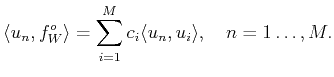
With this initial estimation we `predict' the normal equations (31) and select as our first constraint the worst predicted by the initial solution, let this equation be the $\ell_1$-th one. We then minimize $\sum_{i=1}^M \vert c_i\vert^q$ subject to the constraint

$$\langle u_{\ell_1} , f_{\cal{W}}^o \rangle =\sum_{i=1}^M c_i \langle u_{{\ell_1}} , u_i\rangle ,$$ (33)

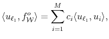
and indicate the resulting coefficients as $c_i^{(1)}, i=1,\ldots,M$. With these coefficients we predict equations (31) and select the worst predicted as a new constraint to obtain $c_i^{(2)}, i=1,\ldots,M$ and so on. The iterative process is stopped when the condition (30) is reached.

The numerical example discussed next has been solved by recourse to the method for minimization of the $(q$-norm)$^q$ published in [16]. Such an iterative method, called FOCal Underdetermined System Solver (FOCUSS) in that publication, is straightforward implementable. It evolves by computation of pseudoinverse matrices, which under the given hypothesis of our problem, and within our recursive strategy for feeding the constraints, are guaranteed to be numerically stable (for a detailed explanation of the method see [16]). The routine for implementing the proposed strategy is ALQMin.m.

This project is supported by EPSRC (EP/D062632/1)