Possible constructions of oblique projector

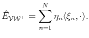
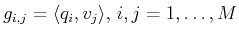
Notice that the oblique projector onto ${\cal{V}}$ is independent of the selection of the spanning set for ${\cal{W}}$ . The possibility of using different spanning sets yields a number of different ways of computing $\hat{E}_{{\cal{V}}{\cal{W}^\bot}}$ , all of them theoretically equivalent, but not necessarily numerically equivalent when the problem is ill posed.

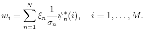
Given the sets $\{v_i\}_{i=1}^{M}$ and $\{u_i\}_{i=1}^{M}$ we have considered the following theoretically equivalent ways of computing vectors $\{w_i\}_{i=1}^{M}$ .

i)

$w_i= \sum_{j=1}^{M} \tilde g_{i,j} u_j$ , where $\tilde g_{i,j}$ is the

-th element of the inverse of the matrix

having elements $g_{i,j}= \langle u_i, v_j\rangle , i,j=1,\ldots,M$ .

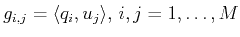
ii)

Vectors $\{w_i\}_{i=1}^{M}$ are as in i) but the matrix elements of

are computed as $g_{i,j}= \langle u_i, u_j\rangle , i,j=1,\ldots,M$ .

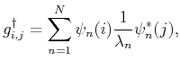
iii)

Orthonormalising $\{u_i\}_{i=1}^{M}$ to obtain $\{q_i\}_{i=1}^{M'} M'\le M$ vectors $\{w_i\}_{i=1}^{M}$ are then computed as

$\displaystyle w_i= \sum_{j=1}^{M} \tilde g_{i,j} q_j,$

with $g_{i,j}= \langle q_i, v_j\rangle , i,j=1,\ldots,M$ .

iv)

Same as in iii) but $g_{i,j}= \langle q_i, u_j\rangle , i,j=1,\ldots,M$ .

Moreover, considering that $\psi_n \in \mathbb{F}^M, n=1,\ldots,M$ , are the eigenvectors of $\hat{G}$ and assuming that there exist

nonzero eigenvalues on ordering these eigenvalues in descending order $\lambda_n, n=1,\ldots,N$ , we can express the matrix elements of the Moore-Penrose pseudo inverse of

as:

$\displaystyle {g}^\dagger_{i,j} = \sum_{n=1}^N \psi_n(i) \frac{1}{\lambda_n} \psi_n^\ast(j ),$

(10)

with $\psi_n(i)$ the

-th component of $\psi_n$ . Moreover, the orthonormal vectors

$\displaystyle \xi_n= \frac{\hat{W}\psi_n}{\sigma_n},\quad \sigma_n=\sqrt{\lambda_n},\quad n=1,\ldots,N$

(11)

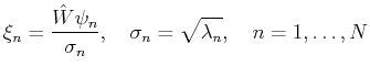
are singular vectors of $\hat{W}$ , which satisfies $\hat{W}^\ast \xi_n=\sigma_n \psi_n$ , as it is immediate to verify. By defining now the vectors $\eta_n, n=1,\ldots,N$ as

$\displaystyle \eta_n= \frac{\hat{V}{\psi_n}}{\sigma_n}, \quad n=1,\ldots,N,$

(12)

the projector $\hat{E}_{{\cal{V}}{\cal{W}^\bot}}$ in (3) is recast

$\displaystyle \hat{E}_{{\cal{V}}{\cal{W}^\bot}}=\sum_{n=1}^N \eta_n \langle \xi_n , \cdot \rangle .$

(13)

Inversely, the representation (3) of $\hat{E}_{{\cal{V}}{\cal{W}^\bot}}$ arises from (13), since

$\displaystyle w_i= \sum_{n=1}^N \xi_n \frac{1} {\sigma_n} \psi^\ast_n(i), \quad i=1,\ldots,M.$

(14)

Proposition 2 The vectors $\xi_n \in {\cal{W}}, n=1,\ldots,N$ and $\eta_n \in {\cal{V}}, n=1,\ldots,N$ given in (11) and (12) are biorthogonal to each other and span ${\cal{W}}$ and ${\cal{V}}$ , respectively.

The proof of this proposition can be found in [7] Appendix A.

All the different numerical computations for an oblique projector discussed above can be realized with the routine ObliProj.m.

Highly Nonlinear Approximations for Sparse Signal Representation

Possible constructions of oblique projector